Download the notebook here!
Interactive online version: ![]()
Outlier Detection in Sensor Data using Functional Depth Measures
Notebook by Jakob R. Jürgens - Final project for the course OSE - Data Science in the summer semester 2021 - Find me at jakobjuergens.com
The best way to access this project is to clone this repository and execute the jupyter notebook and the shiny app locally. Alternatively, on the main site of this repository, there are nbviewer and binder badges set up to directly look at them in the browser.
The following packages and their dependencies are necessary to execute the notebook and the shiny app. If you are executing the code locally, make sure that these packages are provided and that an R Kernel (like irkernel) is activated in the Jupyter notebook.
[1]:
suppressMessages(library(MASS))
suppressMessages(library(tidyverse))
suppressMessages(library(shiny))
suppressMessages(library(shinydashboard))
suppressMessages(library(largeList))
suppressMessages(library(parallel))
suppressMessages(library(Rcpp))
suppressMessages(library(repr))

options(repr.plot.width=30, repr.plot.height=8)

# suppressMessages(library(gganimate)) #needed only to generate the gifs

source("auxiliary/observation_vis.R")
source("auxiliary/distribution_vis.R")
source("auxiliary/updating_vis.R")
source("auxiliary/generate_set_1.R")
source("auxiliary/generate_set_2.R")
source("auxiliary/generate_set_3.R")

sourceCpp('auxiliary/rcpp_functions.cpp')
Table of Contents
Introduction
This project is part of a cooperation with Daimler AG and deals with outlier detection in sensor data from production processes. Since this project will take place over the courses OSE - Data Science (summer semester 2021) and OSE - Scientific Computing for Economists (winter semester 2021/2022), the current state of the project can be seen as a description of the progress at the half time point. Much of the following will be developed further and is therefore subject to change in future revisions.
The main data set that is used in this project deals with the relation of angle and torque during the process of tightening a bolt in a screwing connection. The corresponding data set will be called “Endanzugsproblem” in the following notebook and contains ~350000 observations of what can be imagined as a function that maps angles to torque. The following schematic will give an idea of what the data set represents and what the problem is:
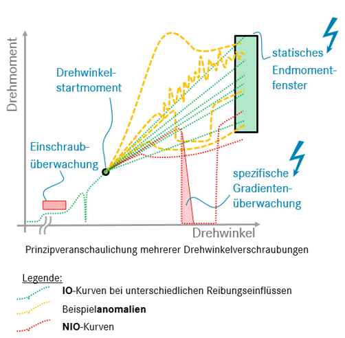
To clarify some things about this simplified schematic:
The so called Endanzug is only part of the tightening process, but the parts of the observation happening before it are not subject of this analysis
The focus of this project lies on curves that are “In Ordnung”, so observations that do not immediately disqualify themselves in some way by for example not reaching the fixed window of acceptable final values
The observations typically have a high frequency of measuring torque, but the measuring points are not equidistant
The angles where torque is measured are not shared between observations, but the measuring interval of angles might overlap between observations
The Endanzug does not start at the same angle for every observation and also does not necessarily start at the same torque
Outliers can be very general, so methods based on detecting only specific types of outliers may not be able to effectively filter out other suspicious observations. So the optimum would be to have some kind of Omnibus test for outliers
Especially due to the high frequency of measurement and the non-identical points where torque is measured, the idea of interpreting each observation as a function and therefore approaching the problem from a standpoint of functional data analysis comes to mind. One method that is used in functional data analysis to identify outliers is based on what is called a “functional depth measure”. Gijbels and Nagy (2017) introduces the idea of depth as follows and then elaborate on the theoretical properties a depth function for functional data should possess:
For univariate data the sample median is well known to be appropriately describing the centre of a data cloud. An extension of this concept for multivariate data (say p-dimensional) is the notion of a point (in \(\mathbb{R}^p\)) for which a statistical depth function is maximized.
The idea is to define an analogous concept to centrality measures (such as the distance from some central tendency like the median) in a scalar setting for functional data and then use those to determine which functions in a set are typical for the whole population. Due to the more applied nature of this project, I will not go into detail on the theoretical properties of the methods used, but focus on giving intuition why the chosen methods make sense in this context.
The main inspiration for my approach to the problem of detecting outliers in a data set such as the one described above is the paper “Outlier detection in functional data by depth measures, with application to identify abnormal NOx levels” by Febrero-Bande, Galeano, and Gonzàlez-Manteiga (2008). I am going to first describe their algorithm, then present my extensions and my implementation and finally apply it to three simulated data sets mimicking the “Endanzugsproblem” as the original data is property of Daimler AG, which I cannot make public.
Observation Structure
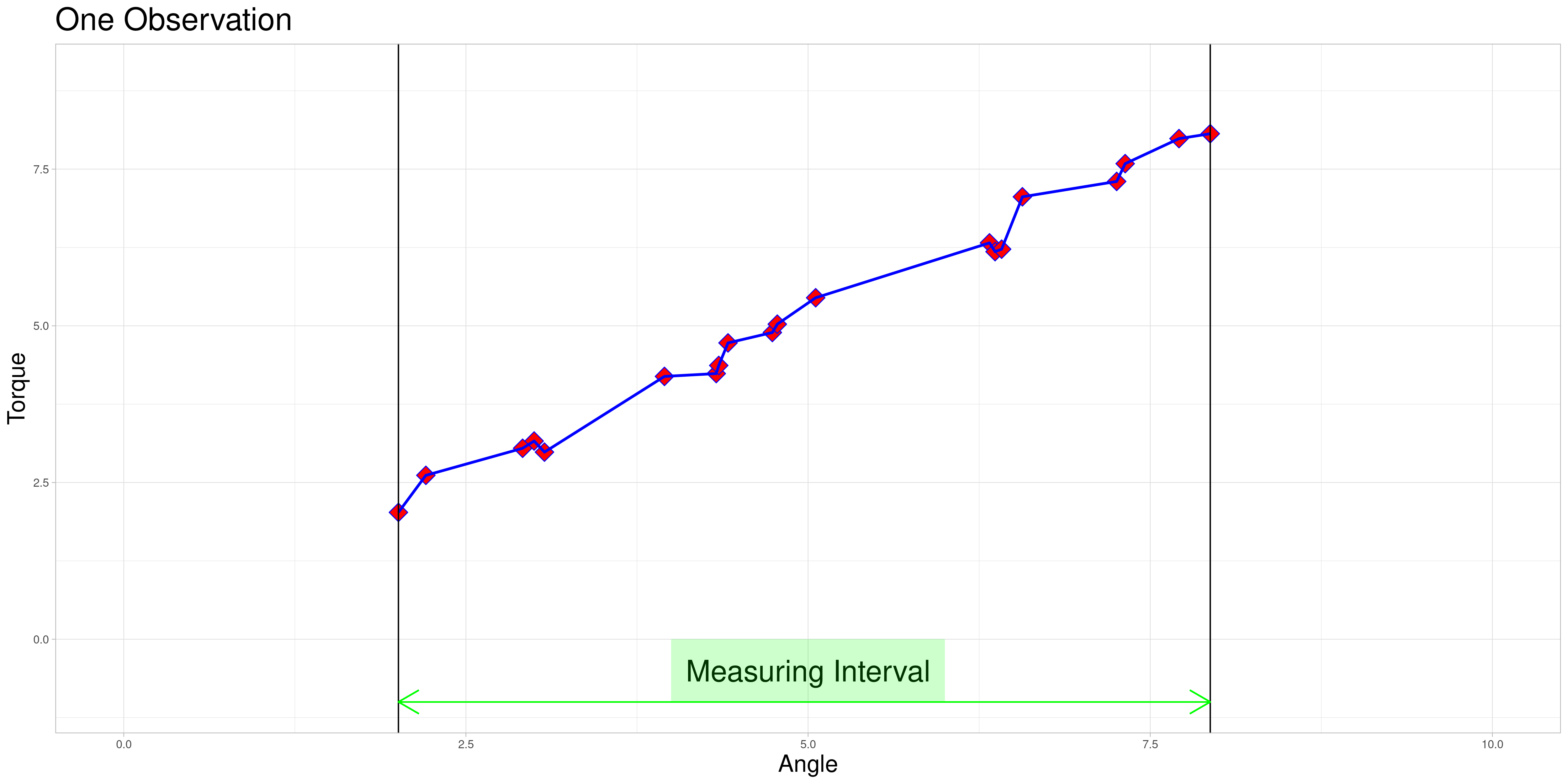
For the sake of clarity, I will show the typical structure of one observation and define a couple of objects I will refer to later. To give context for the later choices of data generating processes, it is useful to know that the physical process of tightening a bolt is typically associated with a linear relationship between angle and torque (at least in the relevant parts of the tightening process) - this approximation is good for the parts of the tightening process that are part of the “Endanzug”. Therefore, simulations in the later parts of this notebook typically assume an approximately linear process as the data generating process for non-outliers.
One observation in a data set might look as follows.
Observation |
1 |
2 |
3 |
4 |
5 |
6 |
7 |
8 |
9 |
10 |
11 |
12 |
13 |
14 |
15 |
16 |
17 |
18 |
19 |
20 |
|---|---|---|---|---|---|---|---|---|---|---|---|---|---|---|---|---|---|---|---|---|
Angle |
2.01 |
2.21 |
2.91 |
3.00 |
3.07 |
3.95 |
4.33 |
4.35 |
4.41 |
4.74 |
4.77 |
5.06 |
6.33 |
6.37 |
6.41 |
6.57 |
7.25 |
7.32 |
7.71 |
7.94 |
Torque |
2.02 |
2.61 |
3.05 |
3.16 |
2.99 |
4.19 |
4.24 |
4.37 |
4.73 |
4.89 |
5.03 |
5.45 |
6.32 |
6.18 |
6.22 |
7.06 |
7.30 |
7.59 |
7.99 |
8.06 |
The red diamonds represent measurements of torque that were taken at a recorded angle.
The blue lines are an example of linear interpolation between the points that were actually measured. This will become important later on.
The measuring interval marked in green is the convex hull of angles where measurements were taken for this observation.
The data set contains many of these objects, that do not necessarily share these characteristics.
[2]:
# Generated using function from auxiliary/observation_vis.R
# source("auxiliary/observation_vis.R")
# obs_vis()
The Algorithm
The idea of Febrero-Bande, Galeano, and Gonzàlez-Manteiga (2008) is an iterative process that classifies observations as outliers if their functional depth lies below a threshold C, which is determined using a bootstrapping procedure in each iteration. The algorithm can be decomposed into two parts:
The iterative process: (quoted from Febrero-Bande, Galeano, and Gonzàlez-Manteiga (2008))
Obtain the functional depths \(D_n(x_i),\: \dots \: ,D_n(x_n)\) for one of the functional depths […]
Let \(x_{i_1},\: \dots,\: x_{i_k}\) be the k curves such that \(D_n(x_{i_k}) \leq C\), for a given cutoff \(C\). Then, assume that \(x_{i_1},\: \dots,\: x_{i_k}\) are outliers and delete them from the sample.
Then, come back to step 1 with the new dataset after deleting the outliers found in step 2. Repeat this until no more outliers are found.
The underlying idea is that observations that are more central in the sense of the chosen depth will have higher depth assigned to them. So choosing the least deep observations from a data set is a reasonable way to search for atypical observations. The question of where to draw the border for observations to be classified as abnormal is done using a bootstrapping procedure described next.
Determining C: (quoted from Febrero-Bande, Galeano, and Gonzàlez-Manteiga (2008))
Obtain the functional depths \(D_n(x_i),\: \dots ,\:D_n(x_n)\) for one of the functional depths […]
Obtain B standard bootstrap samples of size n from the dataset of curves obtained after deleting the \(\alpha \%\) less deepest curves. The bootstrap samples are denoted by \(x_i^b\) for \(i = 1,\: \dots,\: n\) and \(b = 1,\: \dots,\: B\).
Obtain smoothed bootstrap samples \(y_i^b = x_i^b + z_i^b\), where \(z_i^b\) is such that \((z_i^b(t_1), \dots, z_i^b(t_m))\) is normally distributed with mean 0 and covariance matrix \(\gamma\Sigma_x\) where \(\Sigma_x\) is the covariance matrix of \(x(t_1),\: \dots,\: x(t_m)\) and \(\gamma\) is a smoothing parameter. Let \(y_i^b\), \(i = 1,\: \dots,\:n\) and \(b = 1,\:\dots,\: B\) be these samples. *
For each bootstrap set \(b = 1,\:\dots,\:B\), obtain \(C^b\) as the empirical 1% percentile of the distribution of the depths \(D(y_i^b)\), \(i = 1,\: \dots,\: n\).
Take \(C\) as the median of the values of \(C^b\), \(b = 1,\: \dots,\: B\).
This is done, as a theoretical derivation of the distribution of depth values for data generated by a specific data generating process is often infeasible. Instead, one drops a fraction of observations \(\alpha\) and uses a smoothed bootstrapping algorithm to approximate the corresponding threshold value to remove approximately that fraction of observations in the procedure listed under 1.
*At this point in the algorithm the assumption that the functional observations are observed at a set of discrete points \(t_1,\:\dots,\:t_m\) has already been made.
Some important points:
I decided to deviate from the original procedure proposed by the authors by allowing the user to decide whether to reestimate \(C\) in each iteration of the process. The authors present good arguments, why keeping \(C\) fixed is the better approach and my testing confirms those. But to keep the possibilities for experimentation open, I opted to implement it in this way nevertheless. In later stages of this project I will go into detail on why keeping \(C\) constant also has some problems and try to introduce corrections to improve the method developped below.
The authors recommend a choice of \(\gamma = 0.05\) as a smoothing parameter for the bootstrap which I adopted in my applications.
For the choice of \(\alpha\) preexisting information on the data should be used if available. A good way to choose this is the expected fraction of outliers in the data. However, my testing showed that in some cases the choice of this parameter had to be lower than the actual fraction of observations generated by abnormal processes when using a sampling procedure to get better results.
The authors propose three functional depth measures and benchmark them in a simulation setting. Because of their results and the computational cost which are comparatively small, I chose to use h-modal depth for my implementation, which I will introduce in the following.
h-modal depth
Introduced by Cuevas, Febrero-Bande, and Fraiman (2006) h-modal depth is one of three depth measures covered in Febrero-Bande, Galeano, and Gonzàlez-Manteiga (2008). I will follow the summary in the latter paper for my overview. The idea behind this depth is that a curve is central in a set of curves if it is closely surrounded by other curves.
In mathematical terms, the h-modal depth of a curve \(x_i\) in relation to a set of curves \(x_1, \dots, x_n\) is defined as follows:
where \(K: \mathbb{R^{+}} \rightarrow \mathbb{R^{+}}\) is a kernel function and \(h\) is a bandwidth. The authors recommend using the truncated Gaussian kernel, which is defined as follows:
and to choose \(h\) as the 15th percentile of the empirical distribution of \(\{||x_i - x_k|| \, | \, i,k = 1,\:\dots,\:n\}\)
I chose to implement the \(L^2\) norm - one of the norms recommended by the authors - as it performed better than the \(L^{\infty}\) norm (which was also recommended) in my preliminary tests. In a functional setting \(L^2\) is defined by:
where a and b are the boundaries of the measurement interval. This can be replaced by its empirical version
in case of a discrete set of \(m\) observation points shared between observations.
The choice of the functional norm could be adjusted to deal with data resembling different functional forms. This could be part of a possible extension, where different norms are implemented and compared. This might become part of future iteratons of this project.
Difficulties due to the Data
The Endanzug does not start at the same angle for every observation.
In this setting the fact that the first measurement is taken at different angles is not of a problem, since the property of interest is the shape of the curve after the Endanzug has started. In real world terms, the beginning of the “Endanzug” is determined by the first angle where a specific torque is exceeded and the change in torque during the “Endanzug” is of interest and not the position of the “Endanzug” in the whole tightening process. Therefore, all observations can be modified by subtracting the first angle of the “Endanzug” from all angles, effectively zeroing the observations.
At this time, I am going to focus on problems where zeroing is admissible and elaborate on how to possibly extend the method to scenarios where it is not. Those generalizations will be part of further work on this project.
After zeroing, the measurement intervals might still not be identical due to differing lengths.
I decided to try to remedy this remaining problem in the zeroed data set by stretching the measuring intervals to a shared interval while leaving the observed torques identical. Excessive stretching however is problematic, as it can lead to similar observations ending up very different. Putting a conservative limit on stretching should however conserve the quality of relationships between observations. This should lead to limited influence on the calculated depths of the functional observations. To do so, I define a parameter \(\lambda \geq 1\) called acceptable stretching and make observations comparable by stretching their measuring intervals by a factor \(\psi_i \in [1/\lambda, \lambda]\) before approximating them using linear interpolation. In an optimal setting stretching would not be necessary and employing it leads to trade offs, so this parameter should be chosen conservatively.
If zeroing as described in 1. is not appropriate, a combination of acceptable stretching and acceptable shifting could be implemented to increase the size of sets of pairwise comparable functions. This will be part of future extensions of this project.
As you can already see in this animation, the acceptable stretching introduces inaccuracies even in an approximately linear setting. Outlier classifications could be quite sensitive to this parameter.
The angles where torque is measured are not shared between observations.
Assuming that the measuring intervals are identical, I decided to use linear interpolation to approximate the observations. This is done to treat them as if they had been observed at a shared grid of angles to make them compatible with the simplification of the h-modal norm described above. This is only an approximation, but choosing an appropriately fine grid to approximate the observations should limit the influence of this procedure on the calculated functional depths. Espacially in case of the dataset under consideration in this project, performing this approximation by linear interpolation should not result in large distortions due to the linearity of the described physical process. In other settings this approximation could lead to bad performance. One example that came to my mind is if most observations are zero, the frequency of taking measurements is comparatively low and the relevant parts of the observations are instantaneous deviations from zero (or spikes that have infinitesimally small duration). In cases like the one described, it would probably be a better idea to choose a different method or at least choose a different functional norm more appropriate for the dgp due to the necessity of very fine grids to achieve a appropriate approximation of the data. Benchmarking of the method for different data generating processes will be part of future revisions to explore the applicability of the developed method.
For sufficiently smooth processes with a high measuring frequency this approximation should however not result in huge distortions.
Another possibility to approach this third problem would be to use a different version of the norm for discretized points I described above. Instead of calculating
for a set of points on a grid approximated by linear interpolation, one could instead define functions \(\tilde{x}_i\) which are just the piece wise linear functions defined by connecting the observed points of \(x_i\). A norm based on this could be constructed as:
For very fine grid approximations these criteria should result in similar depths, as under some mild conditions, the first approach will converge to the second for increasingly fine grids. In a sense the first approach is similar to a Riemann sum which for increasingly fine grids converges to the corresponding Riemann integral under the necessary assumptions.
Runtime Complexity
The runtime complexity of this algorithm is at least \(O(n^2)\) and I concluded that using my implementation it is infeasible to use it on a very large data set such as the “Endanzugsproblem” (assuming that all observations are comparable at once). Even when splitting up the observations as proposed above into comparable subsets, some of them will be too large to directly approach with this method. To solve this problem, I instead opted to use a sampling approach which I explain in the next section.
[3]:
### The gifs have been rendered using function from auxiliary/observation_vis.R (needs more packages, than are available in this environment)
# source("auxiliary/observation_vis.R")
# stretching_vis()
# zeroing_vis()
# lin_approx_vis()
Sampling Approach
Since it is infeasible to use this method on very large data sets at once, I chose to pursue a sampling-based approach instead. Intuitively this is reasonable as in many cases observations that are atypical in the full data set will be classified as atypical in its subsamples more often than “typical” observations. If this principle does not apply to the data set, a sampling-based approach is difficult to justify. In a case like that it is more reasonable to choose differnet methods to identify abnormal observations.
As the assumption seems reasonable in case of the “Endanzugsproblem”, instead of performing the algorithm described above on the whole data set (or its comparable subsets), I devise a procedure as described in the following:
Let \(\{x_1, \dots, x_L\}\) be a set of observations that are comparable using the algorithm but too large to perform this procedure in reality.
Define the following objects:
Let num_samples
\[= (a_1,\:\dots,\: a_L) \in \mathbb{N}_0^L\]where \(a_i\) is the number of samples \(x_i\) was part of \(\quad \forall i \in \{1,\:\dots,\: L\}\). (Initialize all entries as 0)
Let num_outliers
\[= (b_1,\:\dots,\: b_L) \in \mathbb{N}_0^L\]where \(b_i\) is the number of samples \(x_i\) was classified as an outlier in
\[\quad \forall i \in \{1,\:\dots,\: L\}\]. (Initialize all as entries 0)
Let frac_outliers
\[= (c_1,\:\dots,\: c_L) \in \mathbb{R}_{\geq 0}^L\]where \(c_i = \begin{cases}1 & a_i = 0 \\ \frac{b_i}{a_i} & a_i > 0\end{cases} \quad \forall i \in \{1,\:\dots,\: L\}\) (Initialize all entries as 1)
Draw a sample of size K from \(\{x_1,\: \dots,\: x_L\}\) without replacement
Perform the outlier detection procedure on this sample and update the vectors according to your results.
Go back to two and iterate this process until some condition is fulfilled.
Typical conditions could be:
A specified number of iterations was reached
Every observation was part of more than a specified number of samples
The vector of certainties did not change enough according to some criterion over a specified number of iterations
In the end, the entries of frac_outliers can be used as a metric for the outlyingness of an observation. If a binary decision rule is needed, every observation with an entry over some specified threshold could be classified as an outlier.
Finding Comparable Sets of Observations
Assume for the sake of simplicity that zeroing is reasonable so that the minima of the measurement intervals of the observations are all zero. Therefore, the measurement intervals only differ in their end points or lengths which is identical in this case. As an example to visualize possible ways to find comparable subsets assume that the empirical distribution of endpoints looks as follows:
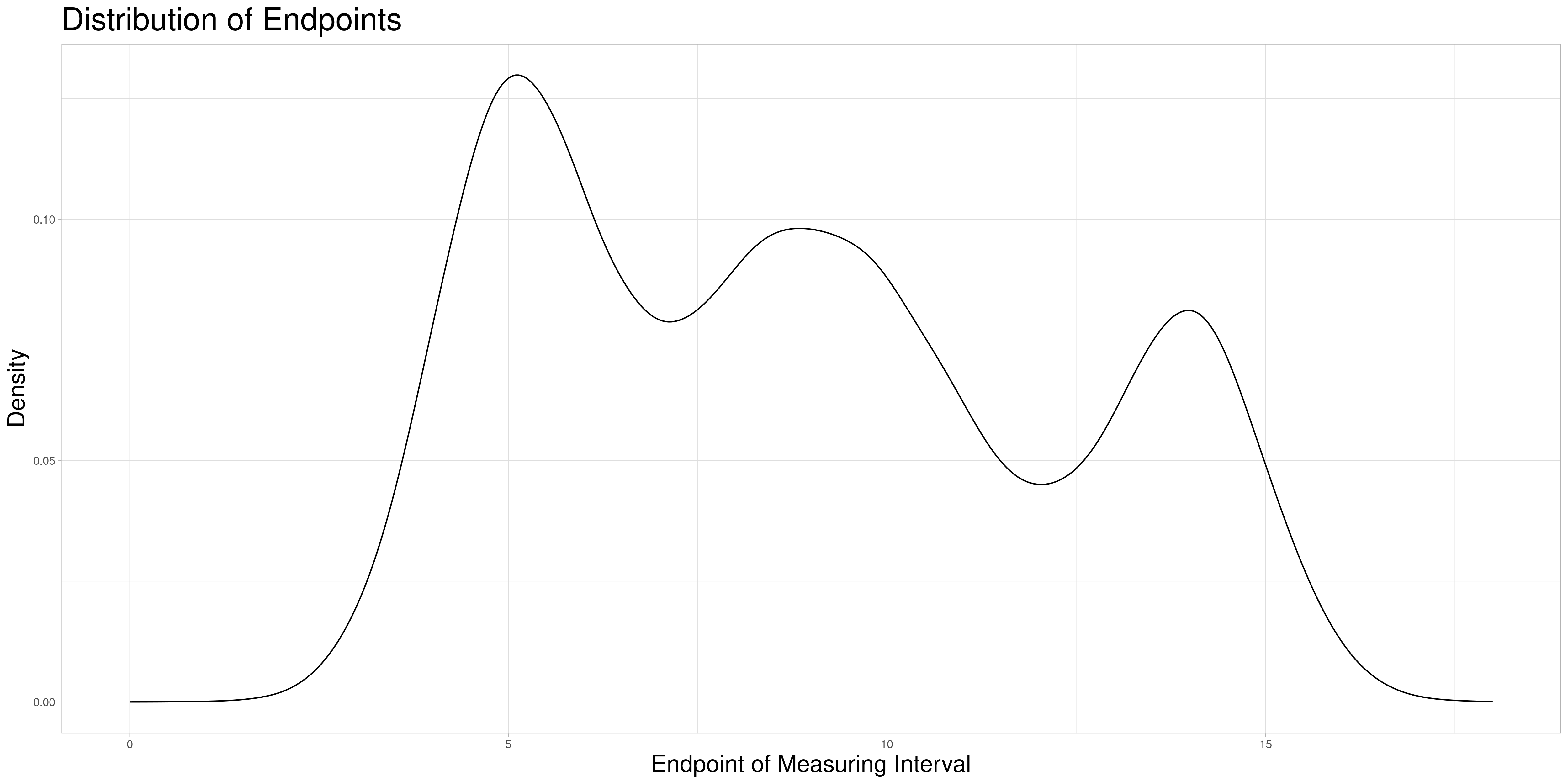
In the following I describe three methods to find comparable subsets to perform the sampling procedure on and explain why I chose the method that I ultimately implemented.
Static Splitting
For Static Splitting the idea is to partition the whole data set into pairwise disjunct subsets of pairwise comparable observations. This partition depends on the acceptable stretching parameter and is not necessarily unique for a choice of the acceptable stretching parameter. Therefore, a choice procedure would have to be introduced if this approach were to be taken. Some possible partitions of the set above (not necessarily consistent with the same acceptable stretching parameter) could look like this:
However, this idea has some problems:
The choice of subsets could introduce a new source of distortions in addition to the acceptable stretching parameter.
Adding new observations could change the chosen subsets, making an updating procedure difficult to realize.
In each individual subset, the observations that are changed due to stretching are identical over samples. This could lead to distortions since for some observations not the original but only the stretched observations are taken into account in the classification.
Dynamic Splitting
This approach has some advantages over the first one:
The choice of subsets becomes only a question of the acceptable stretching parameter and not of the choice of algorithm that chooses the partition of the data set.
Adding new observations is unproblematic, as new observations do not influence the allocation of comparable subsets. Therefore additional samples containing the new observation can be drawn without creating problems in the comparability to previous sampling-based results. A procedure like this is described in the next section.
Each observation can enter the classification procedure undistorted in at least the comparable subset corresponding to its own endpoint. Additionally, it can enter the classification in samples, where it is comparable due to acceptable stretching. The latter can realize for different degrees of stretching - increasing or decreasing the length of the measuring interval. This solves the problem of observations being used for classification only in a specific distorted state.
Dynamic Splitting with varying acceptable stretching parameter
As shown above, the difference in length of these comparable subsets changes quite substantially and does not react to the density of observations having similar measurement intervals. A deviation from this appraoch might be desirable for multiple reasons:
If there are many observations with a very similar measuring interval, including observations with a more dissimilar interval (in terms of the animation above, a midpoint farther away) might be detrimental to the procedure’s performance. If there are fewer observations close by one might want to allow for a bigger acceptable stretching parameter to allow for more comparisons.
In tandem with the advantage above one could also change the sample size to suit specific needs of the procedure.
It would be possible to use a local acceptable stretching parameter that changes as a function of the estimated density of end points (since zeroing was admissible in this example). Using a rather simple function determining the local acceptable stretching parameter to serve as an example leads to the following choice of comparable subsets.
In this example the effect is quite subtle, but in comparison to the previous animation, one can see that the expansion of the interval of end points of comparable observations is slower in regions, where the estimated density of end points is higher. There are two reasons why I decided against making acceptable stretching a varying parameter in my implementation:
It introduces another complication as the function to determine the local acceptable stretching has to be chosen.
It makes the updating procedure described later more difficult, as adding more observations will change the estimated density of the end points and thereby change the comparable subsets.
Choice for Implementation
Due to the advantages and disadvantages described above, I decided to implement Dynamic Splitting with a global acceptable stretching parameter. This makes it easier to later justify an updating procedure and still does not create distorted results as described for Static Splitting.
[4]:
### The graphics and gifs have been rendered using function from auxiliary/observation_vis.R (needs more packages, than are available in this environment)
# source("auxiliary/distribution_vis.R")
# dist_vis()
# static_splits_vis()
# dynamic_splits_vis()
# dynamic_splits2_vis()
Description of Full Procedure for Existing Data sets
Having explained
The algorithm by Febrero-Bande, Galeano, and Gonzàlez-Manteiga (2008)
The sampling approach
The procedure for selecting comparable subsets with dynamic splitting of the data set
I am going to explain the full procedure applied to an existing data set assuming that zeroing is admissible.
Definition of Objects
Let \(x_1,\: \dots,\: x_n\) be the full data set of observations as described in the beginning
Let \(I_1 = [s_1, e_1], \dots, I_n = [s_n, e_n]\) be the measuring intervals of \(x_1, \dots, x_n\)
Assuming that zeroing is admissible:
Let \(\bar{x}_1,\: \dots, \:\bar{x}_n\) be the corresponding zeroed observations
Let \(\bar{I}_1 = [0, \: \bar{e}_1], \: \dots, \bar{I}_n = [0, \bar{e}_n]\) be the corresponding zeroed measuring intervals
Let \(\bar{E} = \{\bar{e} \: | \: \exists k \in \{1, \dots, n\} \: \text{s.t.} \: \bar{e} = \max(\bar{I}_k)\}\) be the set of measuring interval end points occurring in \(\bar{I}_1,\: \dots,\: \bar{I}_n\)
Let \(\bar{\Lambda}(\bar{x}, \bar{e})\) be the resulting object when zeroed observation \(\bar{x}\) is stretched to fit zeroed measuring interval \(\bar{I} = [0, \bar{e}]\)
Again assuming that zeroing is admissible, one can reasonably define the following objects.
Let \(\bar{Z}(\bar{e}, \lambda) = \{\bar{x}_k \: | \: \frac{\bar{e}_k}{\bar{e}} \in [\frac{1}{\lambda},\lambda]\}\) be the set of zeroed observations that can be compared to a zeroed observation with measuring interval \(\bar{I} = [0, \bar{e}]\) with an acceptable stretching factor of \(\lambda\).
Let \(\bar{S}(\bar{e}, \lambda) = \{\bar{\Lambda}(\bar{e}, \bar{x}) \: | \: \bar{x} \in \bar{Z}(\bar{e}, \lambda)\}\) be the set of zeroed observations that have been stretched with an admissible stretching factor to be comparable to a zeroed observation with zeroed measuring interval \(\bar{I} = [0, \bar{e}]\).
If zeroing is not a valid approach, corresponding objects dependent on acceptable shifting and acceptable stretching have to be defined, which will be one challenge in generalizing this method.
Procedure
Choose parameters:
\(\lambda\) acceptable stretching
\(L\) sample size in sampling procedure (may also be varying depending on chosen approach for sampling)*
\(K\) number of equidistant points in grid for approximation by linear interpolation*
\(\alpha\) fraction of observations to drop in approximation of cutoff value \(C\) in outlier classification algorithm*
\(B\) sample size in approximation of cutoff value \(C\) in outlier classification algorithm*
\(\gamma\) tuning parameter in approximation of cutoff value \(C\) in outlier classification algorithm*
Initialize the following vectors:
num_samples
\[= (a_1,\:\dots,\: a_n)\in \mathbb{N}_0^n \quad\]with all entries being 0
num_outliers
\[= (b_1,\:\dots,\: b_n)\in \mathbb{N}_0^n \quad\]with all entries being 0
frac_outliers
\[= (c_1,\:\dots,\: c_n) \in \mathbb{R}_{\geq 0}^n \quad\]with all entries being 1
Iterate through the elements of \(\bar{E}\) doing the following:
Let \(\hat{e}\) be the element of \(\bar{E}\) currently looked at
Determine \(\bar{S}(\hat{e}, \lambda)\) and perform the sampling based outlier identification procedure on this set for some predetermined stopping condition
Update num_samples, num_outliers, and frac_outliers for both the stretched and non-stretched observations in \(\bar{S}(\hat{e}, \lambda)\) as described in the section about sampling
Go to the next element of \(\bar{E}\) and repeat until all elements have been reached.
Report frac_outliers as a measure of outlyingness for the observations.
*not explicitly mentioned in the procedure below
Updating
The procedure described above is constructed to work for a full data set. In a day-to-day setting the data set will not be static. Instead, new observations will be added and it would be a problem, if all calculations had to be done all over again only to incorporate a comparatively small number of new observations.
Instead, I devise mechanisms to assign comparable values of frac_outliers to the newly added observations and to possibly also update the pre-existing observations due to the presence of the newly added ones. In the following assume that new observations are added sequentially. Two ways came to my mind to approach this updating procedure, one more true to the original process (1) and the other one less computationally expensive (2).
Version 1:
This procedure involves additional samples from all sets the new observation could have been part of. So both in a stretched form or in its original form
Let \(x'\) be the new observation and \(\bar{x}'\) its zeroed counterpart. Define \(I'\), \(\bar{I'}\) and \(\bar{e}'\) accordingly.
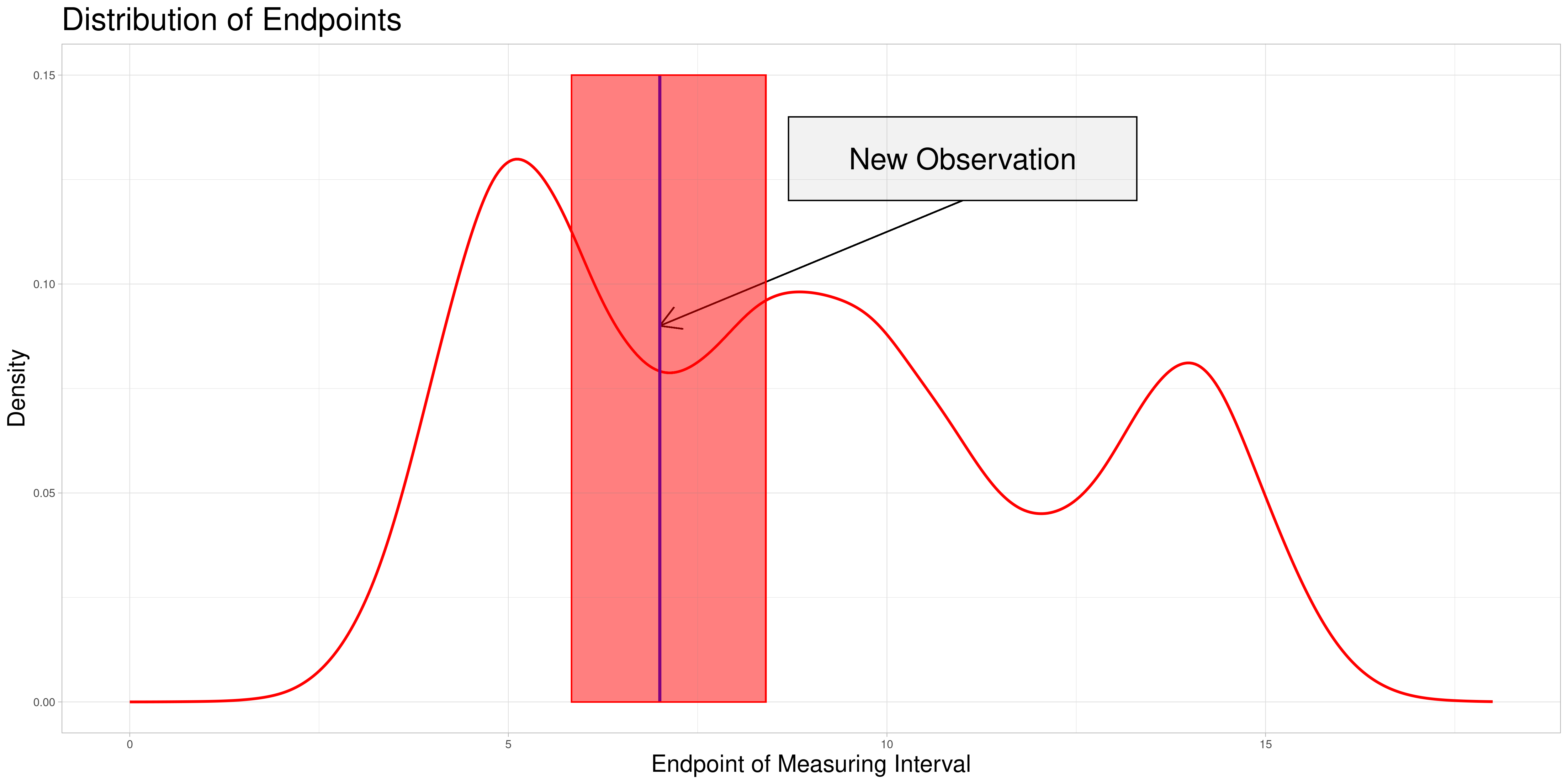
Determine all elements \(\bar{e} \in \bar{E}\) such that \(\bar{x}' \in \bar{Z}(\bar{e}, \lambda)\). Define \(\bar{U}(\bar{x}', \lambda) = \{\bar{e} \in \bar{E} \: | \: \bar{x}' \in \bar{Z}(\bar{e}, \lambda)\}\) as the subset of \(\bar{E}\) called the Updating Window. In this setting where zeroing is admissible, this can be simplified to \(\bar{U}(\bar{x}', \lambda) = \{\bar{e} \in \bar{E} \: | \: \bar{e} \in [\frac{1}{\lambda} \bar{e}', \lambda \bar{e}']\} = \bar{E} \cap [\frac{1}{\lambda} \bar{e}', \lambda \bar{e}']\)
For all \(\tilde{e} \in \bar{U}(\bar{x}', \lambda)\) perform a sampling procedure as follows:
\(\bar{\Lambda}(\bar{x}', \tilde{e})\) is part of each sample
The size of each sample is identical to the one used in the original procedure
The number of samples for each \(\tilde{e}\) is the expected value of the number of samples the new observation would have been part of, if it had been in the original data set
The updating procedure of the vectors works as before. Not only the entry of the new observation in each vector is added and updated, also the entries for the original observations included in the new samples are updated.
So the set of zeroed observations that is potentially updated during this procedure is the following:
Which is visualized in the following animation. (The endpoints of the potentially updated zeroed observations are marked by the red rectangle.)
Version 2:
In comparison the other procedure involves only additional sampling from the set where the new observation is non-stretched.
Let \(x'\) be the new observation and \(\bar{x}'\) its zeroed counterpart. Define \(I'\), \(\bar{I'}\) and \(\bar{e}'\) accordingly.
Determine \(\bar{S}(\bar{e}', \lambda)\) and perform additional sampling as follows:
\(\bar{x}'\) is part of each sample
The number of samples drawn is the expected value of samples the new observation would have been part of, if it had been in the original data set
The updating procedure works as before. Not only the entry of the new observation in each vector is added and updated, also the entries for the original observations are updated.
The following graphic shows the equivalent objects of version 1:
This procedure is less true to the values calculated in the original data set, as the new observation is only taken into consideration in its non-stretched form. Additionally, pre-existing observations could be taken into consideration in their stretched form more frequently depending on the structure of new data being added which could lead to additional distortions. Therefore, I decided to start by implementing the first method and possibly include comparisons of both methods in future revisions.
[5]:
### The graphics and gifs have been rendered using functions from auxiliary/updating_vis.R (needs more packages, than are available in this environment)
# source("auxiliary/updating_vis.R")
# upd_1_vis()
# pot_upd_obs_vis()
# upd_2_vis()
Implementation
I decided to implement these methods in R and C++ and to employ parallelization where possible, to strike a balance between speed and ease of use. C++ functions referenced in the following can be found in /auxiliary/rcpp_functions.cpp. The following section will follow a similar structure as the description of the procedure above ordered as follows:
All of these functions can also be found in /auxiliary/R_functions.R and will in the future be available as an Rcpp-package the tar-ball of which will be included in the repo. In future revisions there will be a secondary notebook with the details of the implementation. This notebook will instead focus on explaining the method and evaluating its perfomance.
Grid Approximation
Finding a grid for Approximation
Assuming that the observations already share the measuring intervals. (Same grid length still acts as a placeholder for a more sophisticated procedure.)
[6]:
# func_dat:

grid_finder <- function(func_dat){
  measuring_interval <- c(min(func_dat[[1]]$args), max(func_dat[[1]]$args))
  return(seq(measuring_interval[1], measuring_interval[2], length.out = 100))
}
Grid approximation by Linear Interpolation
This function acts as a wrapper for a C++ function, that given a vector of arguments, a vector of values and a vector that represents the grid to be used for approximation, performs the desired approximation and returns the vector of approximated values taken at the grid points. This wrapper then combines those values to a matrix, where each row represents the approximated values of an observation at the given grid points.
[7]:
# func_dat: list that contains the observations
# each observation is a list, that conatins two vectors of identical length: args and vals
# grid: grid to use for approximation

grid_approx_set_obs <- function(func_dat, grid) {
  res_mat <- matrix(data = unlist(
      map(.x = func_dat,
          .f = function(obs) grid_approx_obs(obs$args, obs$vals, grid))
    ), nrow = length(func_dat), byrow = TRUE)

  return(res_mat)
}
Sampling Approach
Helper function for parallelization
Since data sets can get large very quickly, it is useful to perform parallelization in this sampling approach in a less memory intensive way. Therefore I decided to write the data set in its prepared form to the disk and use a format that supports random access in lists, to only read in the observations that are part of the sample. After reading in those observations, it performs the outlier detection procedure implemented above.
[12]:
# list_path: path to the random access list of the data set (generated by package largeList)
# index: index of observations to use in the procedure
# alpha: quantile of least deep observations to drop before bootstrapping (in approximation of C)
# B: number of smoothed bootstrap samples to use (in approximation of C)
# gamma: tuning parameter for smoothed bootstrap

random_access_par_helper <- function(list_path, ids, index, alpha, B, gamma){

    # read in the observations identified by the variable index
    func_dat <- readList(file = list_path, index = index)

    # perform the outlier detection procedure on the sample
    # in a tryCatch statement as the procedure creates notamatrix errors in random cases
    sample_flagged <- tryCatch(
        {detection_wrap(func_dat = func_dat, ids = ids, alpha = alpha, B = B, gamma = gamma)},
         error=function(cond){
             return(list(outlier_ids = c(), outlier_ind = c()))}
    )

    # return the object generated by the outlier detection procedure
    return(sample_flagged$outlier_ids)
}
[13]:
# cl: cluster object generated by parallel package
# n_obs: number of observations in data set
# n_samples: number of samples to use
# sample_size: number of observations to use in each sample
# alpha: quantile of least deep observations to drop before bootstrapping (in approximation of C)
# B: number of smoothed bootstrap samples to use (in approximation of C)
# gamma: tuning parameter for smoothed bootstrap
# list_path: path to the random access list of the data set (generated by package largeList)

sampling_wrap <- function(cl, n_obs, n_samples, sample_size, alpha, B, gamma, list_path){

    ids <- 1:n_obs

    # Initialize vectors described in the theoretical section
    num_samples <- rep(x = 0, times = n_obs)
    num_outliers <- rep(x = 0, times = n_obs)
    frac_outliers <- rep(x = 1, times = n_obs)

    # Draw indexes for sampling from functional data without replacement
    sample_inds <- map(.x = 1:n_samples,
                       .f = function(i) sample(x = ids, size = sample_size, replace = FALSE))

    # Determine how often each observation appeared in the samples and update the vector
    freq_samples <- tabulate(unlist(sample_inds))
    num_samples[1:length(freq_samples)] <- num_samples[1:length(freq_samples)] + freq_samples

    # Perform the outlier classification procedure on the chosen samples parallelized
    # with the function clusterApplyLB() from the parallel package
    sample_flagged_par <- clusterApplyLB(cl = cl,
                                         x = sample_inds,
                                         fun = function(smpl){
                                             random_access_par_helper(list_path = list_path, ids = ids[smpl],
                                                                      index = smpl, alpha = alpha,
                                                                      B = B, gamma = gamma)})

    # Determine how often each observation were flagged in the samples and update the vector
    freq_outliers <- tabulate(unlist(sample_flagged_par))
    num_outliers[1:length(freq_outliers)] <- num_outliers[1:length(freq_outliers)] + freq_outliers

    # termine fraction of samples each observation was flagged as an outlier in
    certainties <- unlist(map(.x = 1:n_obs,
                              .f = function(i) ifelse(num_samples[i] != 0, num_outliers[i]/num_samples[i], 1)))

    # Return list containing the three central vectors: num_samples, num_outliers, certainties
    return(list(num_samples = num_samples,
                num_outliers = num_outliers,
                certainties = certainties))
}
How to use this function?
Using the function sampling_wrap() is not as straight-forward as using the previous as multiple steps have to be performed before and after using this function to ensure a problem free experience. I will explain the following code fragments in detail, as depending on which operating system a user employs modifications have to be made. For this reason, the code is commented out in these parts, in order not to cause technical problems that are difficult to replicate. The following code segments were written on a Linux machine and will work on UNIX systems. Since forking is not supported under windows, alternatives would have to be used, like using PSOCK-Clusters instead of ForkClusters.
[14]:
# num_cores <- detectCores()
# cl <- makeForkCluster(num_cores)
#
#
# invisible(clusterCall(cl, fun = function() library('largeList')))
# invisible(clusterCall(cl, fun = function() library('Rcpp')))
# invisible(clusterCall(cl, fun = function() library('purrr')))
# invisible(clusterCall(cl, fun = function() library('MASS')))
# invisible(clusterCall(cl, fun = function() sourceCpp('auxiliary/rcpp_functions.cpp')))
#
# clusterExport(cl, varlist = list("grid_approx_set_obs",
#                                  "approx_C", "grid_finder",
#                                  "outlier_iteration", "outlier_detection",
#                                  "detection_wrap", "random_access_par_helper"),
#                                  envir = .GlobalEnv)
#
# sampling_wrap(cl = cl, n_obs = n_obs, n_samples = n_samples,
#               sample_size = sample_size, alpha = alpha, B = B, gamma = gamma,
#               list_path = list_path)
#
# stopCluster(cl)
num_cores() detects the number of logical cores
makeForkCluster() creates a virtual cluster object that can serve as an argument to functions from the parallel package to perform parallelized computations
the clusterCall() calls execute the command inside on each individual node of the virtual cluster to ensure that all necessary packages are loaded in each instance
clusterExport this exports objects from an environment to each of the nodes. These can be functions or objects.
(These last to steps are technically not necessary in case of a fork cluster, but will navigate around some hard to troubleshoot problems that can occur.)
sampling_wrap() performs the actions implemented above on the virtual cluster cl
stopCluster() stops the cluster, to ensure that it does not clog up the system
Dynamic Splitting
Zeroing
To use the dynamic splitting procedure in the previously described settings, it is first necessary to zero all observations. This is implemented for the functional observations and its results should be saved as a separate object for future use.
[15]:
# func_dat: list that contains the observations
# each observation is a list, that contains two vectors of identical length: args and vals

zero_observations <- function(func_dat){
    zeroed_func_dat <- map(.x = func_dat,
                           .f = function(fnc){
                               args = fnc$args - fnc$args[1]
                               return(args = args, vals = fnc$vals)
                           })
    return(zeroed_func_dat)
}
Determine measuring intervals
This function returns a matrix containing in each row the beginning and end point of the measuring interval of the corresponding observation.
[16]:
# func_dat: list that contains the observations
# each observation is a list, that conatins two vectors of identical length: args and vals

measuring_int <- function(func_dat){
    intervals <- matrix(data = unlist(map(.x = func_dat,
                                          .f = function(obs) c(min(obs$args), max(obs$args)))),
                        nrow = length(func_dat), byrow = TRUE)

    return(intervals)
}
Create a list of measuring intervals that occur in the data set
This set is needed later on for iterating through all possible realizations of the measuring interval to determine the comparable sets for each one.
[17]:
# measuring_intervals: use output from measuring_int()

unique_intervals <- function(measuring_intervals){

    # for finding unique entries transforming to a list is easier
    interval_list <- map(.x = seq_len(nrow(measuring_intervals)),
                         .f = function(i) measuring_intervals[i,])

    # find unique entries
    unique_intervals <- unique(interval_list)

    # combine into matrix again
    unique_matrix <- matrix(data = unlist(unique_intervals),
                            nrow = length(unique_intervals),
                            byrow = TRUE)

    # return matrix where each row contains the beginning and end points of a unique measuring interval
    # from the data set
    return(unique_matrix)
}
Find comparable observations for one measuring interval
Given a measuring interval that is currently under consideration and the matrix of all measuring intervals, determine the indices of the observations that are comparable given an acceptable stretching factor \(\lambda\). Here zeroing is assumed, such that the condition simplifies to a condition on the endpoint of the intervals.
[18]:
# main_interval: vector of two elements: starting and end point of measuring interval
# measuring_intervals: use output from measuring_int()
# lambda: acceptable stretching parameter
# ids: identifiers of individual observations

comparable_obs_finder <- function(main_interval, measuring_intervals, lambda, ids){

    # Determine comparable observations by checking interval endpoints
    comparable <- which(measuring_intervals[,2] >= main_interval[2]/lambda
                        & measuring_intervals[,2] <= main_interval[2]*lambda)

    # Return the correspoding indices and the ids of the comparable observations
    return(list(ind = comparable,
                ids = ids[comparable]))
}
This function can then be used for determining which sets to sample from using the sampling procedure implemented above while iterating through the measuring intervals that occur in the data set.
Full Procedure
Stretching an observation
The first function needed for the full procedure is the ability to stretch an observation to be comparable to another.
[19]:
# obs: a list that conatins two vectors of identical length: args and vals
# measuring_interval: a vector with 2 elements, the start and end points of the desired measuring interval

stretch_obs <- function(obs, measuring_interval){

    # calculate stretching factor
    phi <- (measuring_interval[2] - measuring_interval[1]) / (max(obs$args) - min(obs$args))

    # stretch arguments by appropriate factor
    args_stretched <- obs$args * phi

    # return in the format for functional observations
    return(list(args = args_stretched,
                vals = obs$vals))
}
Stretching a set of observations to prepare sampling procedure
This function acts as a wrapper for the previous function and applies it to a set of observations that are stretched to the same measuring interval.
[20]:
# func_dat: list that contains the observations
# each observation is a list, that conatins two vectors of identical length: args and vals
# measuring_interval: a vector with 2 elements, the start and end points of the desired measuring interval

stretch_data <- function(func_dat, measuring_interval){

    # apply function stretch_obs() to each observation in the data set
    stretch_dat <- map(.x = func_dat,
                       .f = function(obs) stretch_obs(obs = obs, measuring_interval = measuring_interval))

    # return list of stretched observations
    return(stretch_dat)
}
Performing stretching and sampling procedure on set of observations
This is nearly identical to the functions for the sampling procedure itself and could easily be included as a subcase. For the sake of clarity, I nevertheless decided to make these separate functions. Understanding the sampling procedure and the stretching functions will make these functions easy to understand.
[21]:
# list_path: path to the random access list of the data set (generated by package largeList)
# index: index of observations to use in the procedure
# alpha: quantile of least deep observations to drop before bootstrapping (in approximation of C)
# B: number of smoothed bootstrap samples to use (in approximation of C)
# gamma: tuning parameter for smoothed bootstrap
# measuring_interval: a vector with 2 elements, the start and end points of the desired measuring interval

random_access_par_stretch_helper <- function(list_path, ids, index, alpha, B, gamma, measuring_interval){

    # read in the observations identified by the variable index
    func_dat <- stretch_data(func_dat = readList(file = list_path, index = index),
                             measuring_interval = measuring_interval)

    # perform the outlier detection procedure on the sample
    # in a tryCatch statement as the procedure creates notamatrix errors in random cases
    sample_flagged <- tryCatch(
        {detection_wrap(func_dat = func_dat, ids = ids, alpha = alpha, B = B, gamma = gamma)},
         error=function(cond){
             return(list(outlier_ids = c(0), outlier_ind = c(0)))}
    )

    # return the object generated by the outlier detection procedure
    return(sample_flagged$outlier_ids)
}
This function performing the parallelized sampling is again very similar. It only differs in four points:
argument measuring_interval: interval the observations are stretched to
argument comparable: ids of the observations to include in the process as now not all observations are to be sampled in the same process
no argument n_obs: this can be replaced by comparable
use of the appropriately changed helper function for the parallelization
Be careful when using the following function. The vectors that are returned only relate to the set of comparable observations currently under consideration. A value of 3 in the first entry of num_samples means that the first observation of the whole data set occurred in 3 samples, not that the first observation from the set of comparable observations occurred in 3 samples. This has to be kept in mind while later using the output of this function.
[22]:
# cl: cluster object generated by parallel package
# n_samples: number of samples to use
# sample_size: number of observations to use in each sample
# alpha: quantile of least deep observations to drop before bootstrapping (in approximation of C)
# B: number of smoothed bootstrap samples to use (in approximation of C)
# gamma: tuning parameter for smoothed bootstrap (in approximation of C)
# list_path: path to the random access list of the data set (generated by package largeList)
# measuring_interval: a vector with 2 elements, the start and end points of the desired measuring interval
# comparable: vector with the indices of comparable observations in the largelist

stretch_and_sample <- function(cl, n_samples, sample_size, alpha, B, gamma, list_path, measuring_interval, comparable, n_obs){

    ids <- comparable

    # Initialize vectors described in the theoretical section
    num_samples <- rep(x = 0, times = n_obs)
    num_outliers <- rep(x = 0, times = n_obs)

    # Draw indexes for sampling from functional data without replacement
    sample_inds <- map(.x = 1:n_samples,
                       .f = function(i) sample(x = ids, size = sample_size, replace = FALSE))

    # Determine how often each observation appeared in the samples and update the vector
    freq_samples <- tabulate(unlist(sample_inds))
    num_samples[1:length(freq_samples)] <- num_samples[1:length(freq_samples)] + freq_samples

    # Perform the outlier classification procedure on the chosen samples parallelized
    # with the function clusterApplyLB() from the parallel package
    sample_flagged_par <- clusterApplyLB(cl = cl,
                                         x = sample_inds,
                                         fun = function(smpl){
                                             random_access_par_stretch_helper(list_path = list_path, ids = smpl,
                                                                              index = smpl, alpha = alpha, B = B, gamma = gamma,
                                                                              measuring_interval = measuring_interval)})

    # Determine how often each observation were flagged in the samples and update the vector
    freq_outliers <- tabulate(unlist(sample_flagged_par))
    num_outliers[1:length(freq_outliers)] <- num_outliers[1:length(freq_outliers)] + freq_outliers

    # Return list containing the three central vectors: num_samples, num_outliers, certainties
    return(list(num_samples = num_samples,
                num_outliers = num_outliers))
}
Putting the pieces together
Now that there are functions that
Find the set of measuring intervals that occur in the data set
Find comparable observations given a specific measuring interval and an acceptable stretching factor
Perform the sampling procedure with acceptable stretching on comparable subsets of the data set
it is possible to assemble the pieces into one cohesive function that performs the outlier classification procedure described above on a data set where zeroing is admissible.
[23]:
# cl: cluster object generated by parallel package
# list_path: path to the random access list of the data set (generated by package largeList)
# measuring_intervals: matrix of measuring intervals
# n_obs: number of observations in the data set
# lambda: acceptable stretching parameter
# n_samples: number of samples to use in each iteration (NULL for procedure determining value)
# sample_size: number of observations to use in each sample in each iteration (NULL for procedure determining value)
# alpha: quantile of least deep observations to drop before bootstrapping (in approximation of C) (NULL for procedure determining value)
# B: number of smoothed bootstrap samples to use (in approximation of C) (NULL for procedure determining value)
# gamma: tuning parameter for smoothed bootstrap (in approximation of C)

dectection_zr_smpl <- function(cl, list_path, measuring_intervals, n_obs, lambda, n_samples = NULL, sample_size = NULL, alpha = NULL, B = NULL, gamma = 0.05){

    # generate useful identifies for vectors
    ids <- 1:n_obs

    # create vectors as described in the description part
    num_samples <- rep(x = 0, times = n_obs)
    num_outliers <- rep(x = 0, times = n_obs)
    frac_outliers <- rep(x = 1, times = n_obs)

    # determine unique intervals to iterate through
    unique_intervals <- unique_intervals(measuring_intervals)
    n_intervals <- dim(unique_intervals)[1]

    # iteration process
    for(i in 1:n_intervals){

        # Possible output
        # print(paste0(i, " out of ", n_intervals))

        # find comparable observations
        comparable <- comparable_obs_finder(main_interval = unique_intervals[i,],
                                            measuring_intervals = measuring_intervals,
                                            lambda = lambda, ids = ids)$ids

        # do stretching and sampling procedure on current comparable observations
        intv_res <- stretch_and_sample(cl = cl, n_samples = n_samples, sample_size = sample_size,
                                       alpha = alpha, B = B, gamma = gamma, list_path = list_path,
                                       measuring_interval = measuring_intervals[i,], comparable = comparable,
                                       n_obs = n_obs)

        # update the vectors
        num_samples <- num_samples + intv_res$num_samples
        num_outliers <- num_outliers + intv_res$num_outliers
    }

    # calculate the relative frequency of outliers
    frac_outliers <- unlist(map(.x = 1:n_obs,
                                .f = function(i) ifelse(num_samples[i] != 0, num_outliers[i]/num_samples[i], 1)))

    # Return the three vectors
    return(list(num_samples = num_samples,
                num_outliers = num_outliers,
                certainties = frac_outliers))
}
Updating
The updating procedure is currently incomplete but will be finalized in future revisions of this project.
Find measuring intervals with possible occurences of new observation
[24]:
# new_func_obs: list with two elements: vectors of equal length called args and vals
# new_id: identifier for the new observation (be careful not to create duplicates - for example just consecutive intergers would be fine)
# list_path: path to the largeList object, where data set is saved
# id_path: path to the RDS file with the identifiers

obs_append <- function(new_func_obs, new_id, list_path, id_path){

    # read in previous ids
    ids <- readRDS(file = id_path)
    # append new ID
    new_ids <- c(ids, new_id)
    # overwrite old ID file
    saveRDS(object = new_ids, file = id_path)

    # largeLists support appending
    saveList(object = list(new_func_obs), file = list_path, append = TRUE)
}
Appending observation to list of functional data and ids
[25]:
# new_func_obs: list with two elements: vectors of equal length called args and vals
# unique_intervals: matrix containing measuring intervals that occur in the data set (one in each row)
# lambda: acceptable stretching parameter

possible_occurences <- function(new_func_obs, unique_intervals, lambda){

    # determine measuring interval of new observation
    new_measuring_interval <- c(min(new_func_obs$args),  max(new_func_obs$args))

    # determine for all previously used measuring intervals if the new
    # observation could have been part of the stretching and sampling procedure
    occurs <- map(.x = 1:(dim(unique_intervals)[1]),
                      .f = function(i) ifelse(new_measuring_interval[2] >= unique_intervals[i,2]/lambda
                                              & new_measuring_interval[2] <= unique_intervals[i,2]*lambda,
                                              TRUE, FALSE))

    # return the indices and intervals that the new observation could have been a part of
    return(list(occurs = occurs,
                occurs_intervals = unique_intervals[occurs, ]))
}
Determine expected number of occurences in this measuring interval sampling run
[26]:
# orig_n_obs: number of observations in the original comparable set (use output from comparable_obs_finder to determine this)
# orig_n_samples: number of samples drawn in the original procedure (this can be updated by adding those drawn now for future updates)
# orig_sample_size: sample size used in the original prrocedure for this comparable subset

exp_num_samples <- function(orig_n_obs, orig_n_samples, orig_sample_size){

    # determine the probability that the observation would have been part of any original sample,
    # if it had been part of the data set
    # exp_per_sample <- choose(orig_n_obs, orig_sample_size - 1) / choose(orig_n_obs + 1, orig_sample_size)
    # simplifies to:
    exp_per_sample <- orig_sample_size / orig_n_obs

    # multiplay with the number of samples and return the number rounded to the next whole integer
    return(ceiling(orig_n_samples * exp_per_sample))
}
Update one measuring interval
work in progress
[ ]:
Updating for one new observation
work in progress
[27]:
obs_update <- function(cl, new_func_obs, list_path, measuring_intervals, lambda, n_samples = NULL,
                       prev_num_samples, prev_num_outliers, sample_size = NULL, alpha = NULL, B = NULL,
                       gamma = 0.05){

    main_interval <- c(min(new_func_obs$args),  max(new_func_obs$args))

    comparable <- comparable_obs_finder

}
Simulated Data
To show possible usecases of the implementation I create three datasets:
No sampling This data set shows the outlier classification procedure of Febrero-Bande, Galeano, and Gonzàlez-Manteiga (2008) in action. It is characterized by:
Observations with identical measuring intervals
Relatively few observations meaning that the algorithm can be applied without sampling
Sampling A data set where observations share the measuring interval but which is large enough that sampling is necessary to use the algorithm
Full procedure
A dataset where observations share the starting point of the measuring interval but have different endpoints.
This is meant to show the full procedure on a data set that is effectively already zeroed.
The functional form of the non-outliers in these data sets is approximately linear which has two reasons:
Simplicity
The approximate linearity of the relationship that is fundamental to the main data set explored in this project (angle and torque when tightening a bolt).
All of these data sets and the results of the outlier classification procedures applied to them can be seen in the shiny app provided in the repository.
No sampling:
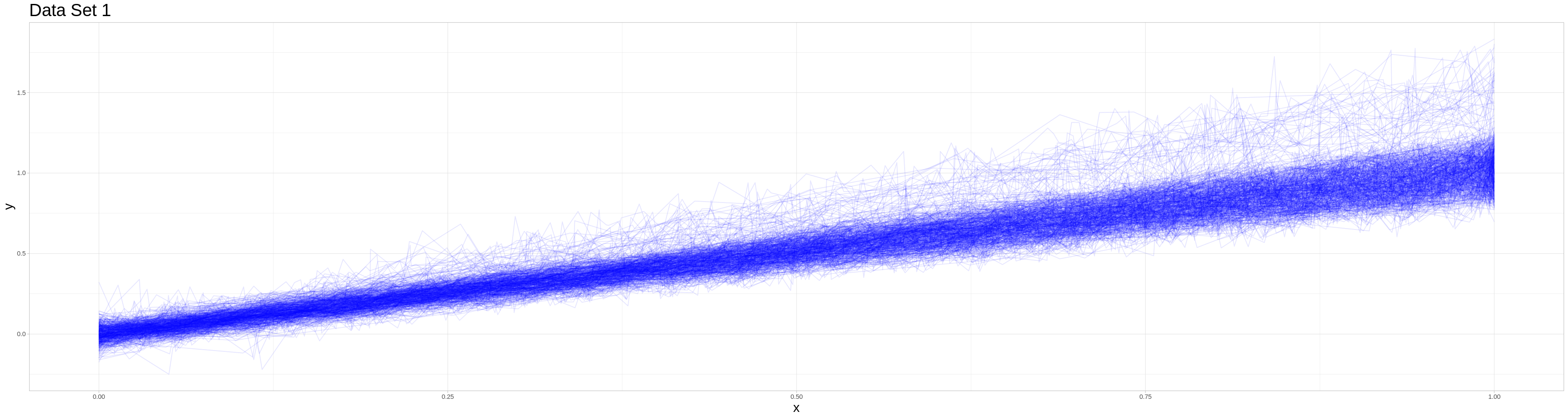
This data set is based on a simple data generating process. Each of the 500 observations is generated as follows:
Determine if the observation is generated as an outlier by drawing from a Bernoulli distributed random variable with parameter 0.05.
Determine the number of points \(k\) where the function is observed. (In the terms of the method above the number of points where measurements are taken) This is drawn from a discrete uniform with elements \(10, \dots, 100\)
The generation of dependent variables depends on whether the observation is generated as an outlier. The general process is as follows:
Draw k-2 realizations of \(p \sim U[0, 1] \quad \text{s.t.} \quad p_1, \dots, p_k \quad \text{i.i.d.}\quad\) Let \(p_{(1)}, \dots, p_{(k-2)}\) be the sorted realizations and define \((0, \: p_{(1)},\: \dots, \: p_{(k-2)},\: 1)^T = \vec{p}\) (This is equivalent to our grid of measuring points.)
Draw k realizations of \(s \sim U[\underset{\bar{}}{s}, \bar{s}] \quad \text{s.t.} \quad s_1, \dots, s_k \quad \text{i.i.d.} \quad\) and define \((s_1,\: \dots, \: s_k)^T = \vec{s}\)
Draw k realizations of \(\epsilon \sim \mathcal{N}[0, \sigma] \quad \text{s.t.} \quad \epsilon_1, \dots, \epsilon_k \quad \text{i.i.d.} \quad\) and define \((\epsilon_1,\: \dots, \: \epsilon_k)^T = \vec{\epsilon}\)
Let \(\vec{y} = m \vec{s} \odot \vec{p} + \vec{\epsilon}\) be the vector of realizations of the dependent variable, where \(\odot\) is the component-wise (or Hadamard) product.
The parameters are different for non-outliers and outliers: For non-outliers: * \(\underset{\bar{}}{s} = 0.8, \quad \bar{s} = 1.2\) * \(\sigma = 0.05\) * \(m = 1.02\)
and for outliers: * \(\underset{\bar{}}{s} = 1, \quad \bar{s} = 1.4\) * \(\sigma = 0.1\) * \(m = 1.2 * 1.02\)
[28]:
# Data generated, transformed and visualized with functions from auxiliary/generate_set_1.R
# Data set is also saved to ./data/Set_1 and if existent read from there instead
# source("auxiliary/generate_set_1.R")

if(file.exists("./data/Set_1/functional.llo") &&
   file.exists("./data/Set_1/ids.RDS") &&
   file.exists("./data/Set_1/outliers.RDS")){
    data_set_1 <- list(data = readList(file = "./data/Set_1/functional.llo"),
                       ids = readRDS(file = "./data/Set_1/ids.RDS"),
                       outliers = readRDS(file = "./data/Set_1/outliers.RDS"))

} else{
    data_set_1 <- generate_set_1()
}

if(file.exists("./data/Set_1/tibble.RDS")){
   tidy_set_1 <- readRDS("./data/Set_1/tibble.RDS")
} else{
   tidy_set_1 <- tidify_1(data_set_1$data, data_set_1$ids)
   saveRDS(object = tidy_set_1, file = "./data/Set_1/tibble.RDS")
}

vis_1(tidy_set_1)
Prepare data for visualization in the shiny app.
[29]:
if(file.exists("./data/Set_1/detection.RDS")){
    set_1_detection <- readRDS("./data/Set_1/detection.RDS")
} else{
    set_1_detection <- detection_wrap(func_dat = data_set_1$data, alpha = 0.05, B = 50, gamma = 0.05, ids = data_set_1$ids)
    saveRDS(object = set_1_detection, file = "./data/Set_1/detection.RDS")
}

if(file.exists("./data/Set_1/summary.RDS")){
    set_1_summary <- readRDS("./data/Set_1/summary.RDS")
} else{

    missed_outliers = setdiff(data_set_1$outliers, set_1_detection$outlier_ind)
    false_outliers = setdiff(set_1_detection$outlier_ind, data_set_1$outliers)

    set_1_summary <- list(flagged = set_1_detection$outlier_ind,
                          original = data_set_1$outliers,
                          missed = missed_outliers,
                          false = false_outliers)

    saveRDS(object = set_1_summary, file = "./data/Set_1/summary.RDS")
}

if(file.exists("./data/Set_1/shiny_tibble.RDS")){
    shiny_tibble_1 <- readRDS("./data/Set_1/shiny_tibble.RDS")
} else{
    shiny_tibble_1 <- tidy_set_1 %>%
        mutate(outlier = ifelse(ids %in% data_set_1$outliers, TRUE, FALSE),
               flagged = ifelse(ids %in% set_1_detection$outlier_ind, TRUE, FALSE))
    saveRDS(object = shiny_tibble_1, file = "./data/Set_1/shiny_tibble.RDS")
}
Sampling:
This second data set consists of 10000 observations where 95% are generated by the same process as the non-outlier variant in the previous data set. So a vector of arguments is drawn from the continuous uniform on \([0,1]\) of random length. Call this vector args in the following description.
But the outliers take 5 different forms each appearing in about one percent of cases. I will describe their data generating processes in mathematical form in the following:
Exactly as the outliers in data set 1.
Sigmoid function: \(\frac{1}{\mathbb{1} + \exp{(-3 * \text{args})}} + \epsilon\) where \(\epsilon\) is a vector of appropriate length containing i.i.d. elements drawn from \(\mathcal{N}(0, 0.05^2)\)
Half sigmoid function: \(\frac{2}{\mathbb{1} + \exp{(-3 * \text{args})}} - \mathbb{1} + \epsilon\) where \(\epsilon\) is a vector of appropriate length containing i.i.d. elements drawn from \(\mathcal{N}(0, 0.05^2)\)
Exponential function: \(\frac{\exp(args) - \mathbb{1}}{e - 1} + \epsilon\) where \(\epsilon\) is a vector of appropriate length containing i.i.d. elements drawn from \(\mathcal{N}(0, 0.05^2)\)
Noise: i.i.d. draws from \(U[0,1]\)
[30]:
# Data generated, transformed and visualized with functions from auxiliary/generate_set_2.R
# Data set is also saved to ./data/Set_2 and if existent read from there instead
# source("auxiliary/generate_set_2.R")

if(file.exists("./data/Set_2/functional.llo") &&
   file.exists("./data/Set_2/ids.RDS") &&
   file.exists("./data/Set_2/outliers.RDS")){
    data_set_2 <- list(data = readList(file = "./data/Set_2/functional.llo"),
                       ids = readRDS(file = "./data/Set_2/ids.RDS"),
                       outliers = readRDS(file = "./data/Set_2/outliers.RDS"))

} else{
    data_set_2 <- generate_set_2()
}

if(file.exists("./data/Set_2/tibble.RDS")){
   tidy_set_2 <- readRDS("./data/Set_2/tibble.RDS")
} else{
   tidy_set_2 <- tidify_2(data_set_2$data, data_set_2$ids)
   saveRDS(object = tidy_set_2, file = "./data/Set_2/tibble.RDS")
}

vis_2(tidy_set_2)
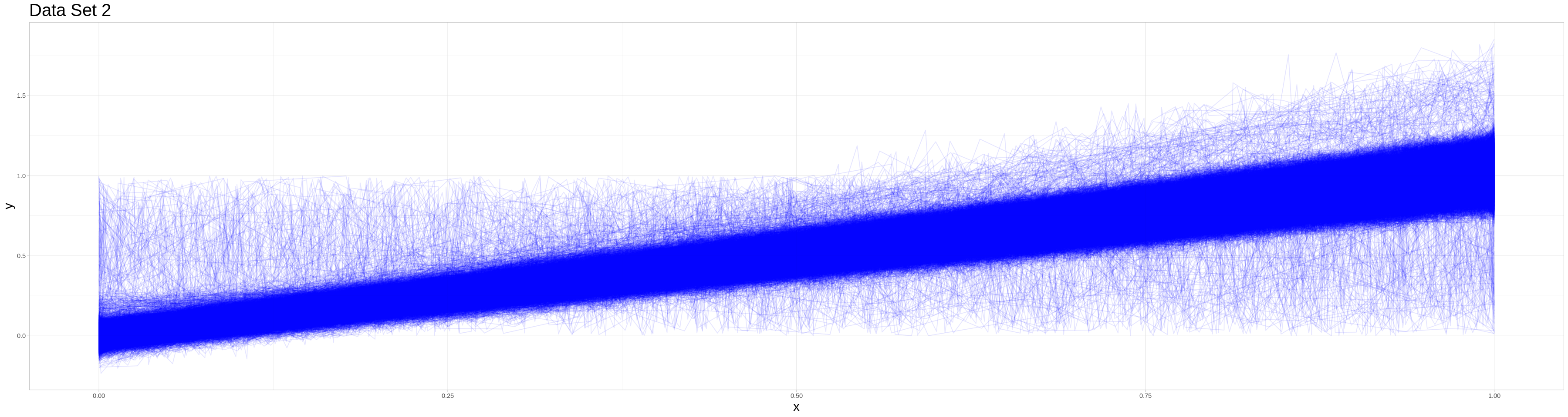
Due to the computational cost of this classifying procedure I saved its results and only perform the classification, if those results could not be found. In the case of 10000 observations can still be done on the full set and I opted to use this lower number of observations not due to computational problems with larger data sets but due to overplotting in the visualizations, that has to be addressed, before large data sets can be appropriately visualized.
[31]:
if(file.exists("./data/Set_2/results.RDS")){
    set_2_results <- readRDS(file = "./data/Set_2/results.RDS")

} else{
    num_cores <- detectCores()
    cl <- makeForkCluster(nnodes = num_cores)

    clusterExport(cl, varlist = list("grid_approx_set_obs",
                                     "approx_C",
                                     "grid_finder",
                                     "outlier_iteration",
                                     "outlier_detection",
                                     "detection_wrap",
                                     "random_access_par_helper"),
                                      envir = .GlobalEnv)

    set_2_results <- sampling_wrap(cl = cl, n_obs = 10000, n_samples = 150,
                               sample_size = 500, alpha = 0.05, B = 100, gamma = 0.05,
                               list_path = "./data/Set_2/functional.llo")

    stopCluster(cl)

    saveRDS(object = set_2_results, file = "./data/Set_2/results.RDS")
}

if(file.exists("./data/Set_2/shiny_tibble.RDS")){
    shiny_tibble_2 <- readRDS("./data/Set_2/shiny_tibble.RDS")
} else{
    shiny_tibble_2 <- tidy_set_2 %>%
        mutate(outlier = ifelse(ids %in% data_set_2$outliers, TRUE, FALSE))

    lengths <- unlist(map(.x = 1:10000,
                          .f = function(i) length(data_set_2$data[[i]]$vals)))

    shiny_tibble_2$cert <- unlist(map(.x = 1:10000,
                                      .f = function(i) rep(set_2_results$certainties[i], times = lengths[i])))

    saveRDS(object = shiny_tibble_2, file = "./data/Set_2/shiny_tibble.RDS")
}
To see the results of this classification procedure for different values of the certainty threshold, you can use the shiny app provided in the repository.
Full Procedure:
This data set is similar to the sampling data set in its data generating process. There are 30000 observations each generated by a similar process as in data set 2.
The main difference is, that the measuring intervals are not identical and are drawn from the following possibilities:
Endpoint of Measuring Interval |
0.9 |
1 |
1.1 |
1.5 |
1.6 |
1.7 |
1.9 |
2 |
2.1 |
|---|---|---|---|---|---|---|---|---|---|
Probability |
0.05 |
0.2 |
0.05 |
0.07 |
0.15 |
0.08 |
0.1 |
0.25 |
0.05 |
Also the data generating processes for both the outliers and the non-outliers are scaled such that the expected realizations at the beginning and end of the data set are identical. (Especially important for the exponential and sigmoidal outliers.) An exception from this are the type 5 outliers, which stay uniformly distributed - but the upper border of the support is made to fit the expected realization of the non-outlier process at the end point of the measuring interval.
[32]:
# Data generated, transformed and visualized with functions from auxiliary/generate_set_3.R
# Data set is also saved to ./data/Set_3 and if existent read from there instead
source("auxiliary/generate_set_3.R")

if(file.exists("./data/Set_3/functional.llo") &&
   file.exists("./data/Set_3/ids.RDS") &&
   file.exists("./data/Set_3/outliers.RDS")){
    data_set_3 <- list(data = readList(file = "./data/Set_3/functional.llo"),
                       ids = readRDS(file = "./data/Set_3/ids.RDS"),
                       outliers = readRDS(file = "./data/Set_3/outliers.RDS"))

} else{
    data_set_3 <- generate_set_3()
}

if(file.exists("./data/Set_3/tibble.RDS")){
   tidy_set_3 <- readRDS("./data/Set_3/tibble.RDS")
} else{
   tidy_set_3 <- tidify_3(data_set_3$data, data_set_3$ids)
   saveRDS(object = tidy_set_3, file = "./data/Set_3/tibble.RDS")
}

### Due to a lengthy plotting time and overplotting, this plot is saved an inserted as a png
# vis_3(tidy_set_3)
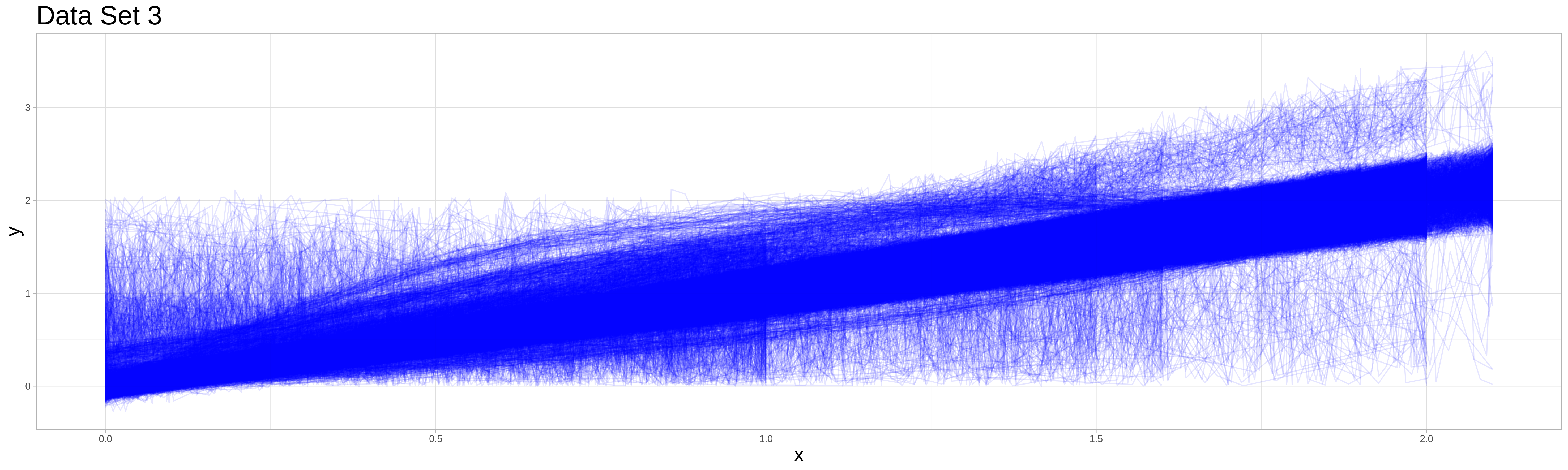
Full procedurre still does not worrk. Produces certainties greater one.
[33]:
if(file.exists("./data/Set_3/results.RDS")){
   set_3_results <- readRDS(file = "./data/Set_3/results.RDS")
} else{
    num_cores <- detectCores()
    cl <- makeForkCluster(nnodes = num_cores)

    clusterExport(cl, varlist = list("grid_approx_set_obs",
                                     "approx_C",
                                     "grid_finder",
                                     "outlier_iteration",
                                     "outlier_detection",
                                     "detection_wrap",
                                     "random_access_par_helper"),
                                      envir = .GlobalEnv)

    measuring_intervals <- measuring_int(func_dat = data_set_3$data)

    comp_test <- comparable_obs_finder(main_interval = c(0,1), measuring_intervals = measuring_intervals,  lambda = 1.2, ids = 1:30000)$ids

    #test <- stretch_and_sample(cl = cl, n_samples = 100, sample_size = 100, alpha = 0.02, B = 100, gamma = 0.05, n_obs = 30000,
    #                           list_path = "./data/Set_3/functional.llo", measuring_interval = c(0,1),
    #                           comparable = comp_test)

    set_3_results <- dectection_zr_smpl(cl = cl, list_path = "./data/Set_3/functional.llo", measuring_intervals = measuring_intervals,
                                        n_obs = 30000, lambda = 1.2, n_samples = 300, sample_size = 300, alpha = 0.02, B = 100, gamma = 0.05)

    stopCluster(cl)

   saveRDS(object = set_3_results, file = "./data/Set_3/results.RDS")
}

if(file.exists("./data/Set_3/shiny_tibble.RDS")){
    shiny_tibble_3 <- readRDS("./data/Set_3/shiny_tibble.RDS")
} else{
    shiny_tibble_3 <- tidy_set_3 %>%
        mutate(outlier = ifelse(ids %in% data_set_3$outliers, TRUE, FALSE))

    lengths <- unlist(map(.x = 1:30000,
                          .f = function(i) length(data_set_3$data[[i]]$vals)))

    shiny_tibble_3$cert <- unlist(map(.x = 1:30000,
                                      .f = function(i) rep(set_3_results$certainties[i], times = lengths[i])))

    saveRDS(object = shiny_tibble_3, file = "./data/Set_3/shiny_tibble.RDS")
}
Shiny App
Instead of presenting the visualizations for the classification procedure in static graphics, I decided to use a shiny web app instead. This has multiple advantages in the setting of this final project, but the main motivation behind it was the use case described to me: An engineer wants to get a preselection of suspicious observations they should have a look at.
In this context, having a raw R file as output without an easy way to interact with it, would not be particularly useful. Instead, being able to run this shiny app on a local server with the precalculated values stored in a database, would be more in line with the idea of the job. This also motivates the features I implemented for the app (and plan to implement in future updates) like:
setting the focus to single observations
changing the plotting window
changing the centrainty threshold for observations to be classified as atypical
etc.
To start the shiny app, I recommend cloning this repository and executing the file app.R locally. This will start the shiny app on a local server. Instead, one can choose to use the binder button on the repo site to start it. Due to a lengthy build process, this is not the recommended way to look at it.
The shiny app serves as the visualization for all results of the previously explained simulation studies and shows what a possible deployment of the method in a real world scenario could look like.
Outlook
Since this project will be continued in the next semester as part of the lecture “OSE - Scientific Computing for Economists” I want to give an outlook on what is to come as part of future revisions of this project.
Finalize Implementation of Updating Procedure
In the current state of the project, the implementation of the updating procedure is incomplete. Future revisions will fill this incompleteness and add simulations to show the process of updating and compare cases where observations were added in an updating procedure to data sets containing them from the beginning. This can serve as a device to check the validity of the updating procedure.
Improvements of Implementation
The implementation above still has some other problems. The most striking is the tendency of the sampling procedure to mark a full sample as atypical, if it contains a lower than expected fraction of atypical observations. I plan to address this by introducing a rescaling factor to the cutoff threshold \(C\) that adjusts for the removal of observations from the sample currently under consideration. This seems reasonable, as adding a new observation to a data set will always increase calculated depths for all observations. Therefore, removing observations can lead to overall lower depths and incrementally lower all observations under the cutoff that determines if they are classified as atypical in a sample. This is not described in the paper this project is based on - so it will make some theoretical work necessary to develop an appropritae correction.
Generalizations
As described in a previous section, the method described in this project for data sets which allow for zeroing of the observations could be generalized by introducing another parameter acceptable shifting in addition to acceptable stretching. This could then be used to define a method that finds comparable subsets in data sets that do not allow zeroing. As this introduces more variables and makes a more sophisticated splitting algorithm necessary, it was out of the scope of this project, but will be addressed in the future.
Parameter Choice
An important part of this procedure will be the choice of its tuning parameters: * In its purest form the algorithm needs a choice for \(\alpha\), \(\gamma\), \(B\) and a grid to use for approximation purposes * Adding sampling adds the choice of sample size and number of samples * The full procedure then additionally needs \(\lambda\)
Some of these like sample size and number of samples could be made dependent on the structure of comparable subsets and even change when switching from one comparable subset to the next. One goal of this could be to make each observation appear in a similar number of samples overall. But other reasonable procedures are possible. Others like \(\alpha\) and \(\lambda\) could be chosen by a simulation method. Constructing a similar but smaller data set with intentionally added outliers to perform cross validation or a similar procedure could be an approach for this case. A more sophisticated and detailed description of this method will be part of future revisions.
Making Results reproducible
Currently, the results of the method are mostly non-reproducible when taking about exact numbers. Qualitative results of the procedure will be similar, but due to randomization in the method the replication of exact numbers is currently not possible. This can be addressed with some work to allow for manually setting seeds in the classification algorithm without sampling and in the choice of samples. Because of parallelization this cannot be done be setting the seed once in the beginning.
Performance Measures for the Algorithm & Benchmarking
Tightly connected to the point of parameter choice is the question of how to measure the performance of the outlier detection procedure in different settings.
First, I am going to look for existing data sets that are commonly used to benchmark outlier classification procedures. The performance of this algorithm in these preclassified settings can serve as grounds for determining in which cases and using which parameter choices the method performs well and compare it to existing methods that are applicable in comparable scenarios.
Second, as can be seen by the previously generated data, an ex ante classification of realizations created by different dgps may not appropriately cover the idea of outlyingness. Some realizations in previous data sets look very typical for the non-outlier dgp and a classification as atypical due to the different dgp could lead to an underestimation of the procedures performance. Therefore, a comparison to established methods can serve as a better tool to judge the effectiveness.
Identifying what contributes to outlyingness of an observation
Once atypical observations in a data set are identified, it is very interesting to see what contributes to their outlyingness in the eyes of the algorithm. To create some ex-post explanation for why a classification decision was made would be a useful tool to inform future real-world decisions or improve the procedure itself by incorporating that information into the mechanism. Some interesting approaches to create an ex-post explanation are the following:
Create slightly altered realizations of an observation that has been marked as an outlier and see what effect different alterations have on its classification (or certainty in case of the sampling-based methods).
Compare locally similar observations that have different outcomes in the overall procedure.
There are more ways to gain information on what features contribute to outlyingness, but due to the current scope of this project, more in-depth considerations of this approach will only be part of future revisions.
Creation of an Rcpp-Package to improve usability
Further iterations of this project will be different in the way the functions are made available. Instead of implementing the functions directly in the main notebook, there will be an additional notebook explaining the implementation and an R package that can be installed directly that contains all functionality provided above. This will make it easier to use the functions in the future.
Improvements to the Shiny App
The visualizations of the shiny app will also undergo considerable overhauls, starting with changes to which observations are plotted when focus is set to a single observation. In this case for example plotting more observations in the close vicinity of the observation might be of greater interest, whereas observations farther away may provide little information of use and could be plotted less frequently to avoid overplotting. There are further improvements planned but due to the interactive process of designing an interface that is meant for direct interaction with the user, it is difficult to predict the exact nature of the changes.
Sources
Cuevas, A. & Febrero-Bande, M. & Fraiman, R. (2006). On the use of bootstrap for estimating functions with functional data. Computational Statistics & Data Analysis. 51. 1063-1074.
Febrero-Bande, M. & Galeano, P. & Gonzàlez-Manteiga, W. (2008). Outlier detection in functional data by depth measures, with application to identify abnormal NOx levels. Environmetrics. 19. 331 - 345.
Gijbels, I. & Nagy, S. (2017). On a General Definition of Depth for Functional Data. Statistical Science. 32. 630-639.
Notebook by Jakob R. Jürgens Final project for the course OSE - data science in the summer semester 2021 Find me at jakobjuergens.com